Part 2 of 2
Prompt optimization for an LLM judge: how to see how much accuracy your prompt leaves unused, and when to stop
2026-11-14 · code and data
Anyone who has optimised a prompt for a classifier knows the feeling. You rewrite a sentence and accuracy goes up a point. You rewrite another and it drops two. After enough rounds there is a folder full of versions and no way to tell whether the model has hit its limit, or the right words just have not turned up yet.
That was my situation with a judge model in production. The way out came from an unexpected place: an experiment with editing the model’s weights.
What you can take from this, in brief:
- A check that tells “the model cannot” from “the prompt does not ask”: a logistic regression on the model’s internal state, compared with the model’s own answers.
- It does not need a large labelled set. Here 200 examples to fit and 200 to score were enough to tell a prompt that wastes a lot from one that wastes almost nothing.
- When the two are within wording noise of each other, stop. Every later gain that was re-scored on fresh data shrank to within noise.
- Wording noise is larger than it looks. The same prompt rewritten five ways gave scores with a standard deviation of 0.016, and 0.041 between best and worst.
- What moved accuracy was plain prompt work: framing the page as untrusted content, spelling out criteria, then writing rules from the judge’s errors. Automated search and clever error selection did not beat it.
The how-to is at the end. This is for anyone who optimises prompts for an LLM that classifies, judges or routes.
The borrowed idea
This is the second half of a story. The first half is “A production LLM’s weights edited almost-by-hand”, which is based on “Sparks of Weight-Space Programming”, a blog post from MIT CSAIL: https://rikiyat.github.io/blog/weight-space-programming/
In that post an LLM, GPT-6 Astra, edits the weights of a small model directly, with no training, and the model’s score on a maths benchmark goes from 7.9 % to 48.1 %. It sounds like magic until you read why. The small model was not that bad at maths. It was stuck in loops, and the edit removed the loop. On a second model, which had no such fault, the same approach did nothing. The authors drew the conclusion themselves:
Editing weights could remove an obstacle that hid an ability, but it could not add an ability the model lacked.
Their editing is not used here. Not a single weight changes in this article. What I took is the distinction: hidden ability or missing ability. Knowing which one you have tells you whether another prompt rewrite can still pay.
The first article tried such an edit on the judge. The edit itself turned out to be the least useful thing in that story. The useful thing was what it exposed: the model’s last internal state already contained the answer. The output just was not using it. And a loss that sits there can be measured.
The judge
AI agents read web pages, and a page can carry text written to hijack the agent. The judge, Gemma 4 26B, reads the page first and answers with a single word: does this text give orders to an AI, or is it clean? A page that only discusses such attacks has to pass, which is where it gets hard.
Everything was tuned on 1,579 labelled texts. Scoring used 1,643 new ones collected afterwards, 579 attacks and 864 harmless real pages among them. The score throughout is AUC, a ranking score: 1.0 is perfect, 0.5 is a coin flip.
The check
Five steps, none of them clever.
- Run your labelled examples through the model with your prompt.
- For each one, keep the model’s last internal state. With llama.cpp the embeddings endpoint returns it.
- Fit a logistic regression on the tuning set’s states and score it on the test set.
- Score the model’s own answers on the same test set.
- Subtract. The difference is the accuracy your prompt leaves unused.
Be careful what you read into the regression’s score. It is what a simple classifier can get out of the model’s state. A mark the prompt could reach. It is not proof of what the model “understands”; more on that at the end.
It needs a model you run yourself, because hosted chat APIs generally do not return internal states. It needs labelled examples, though fewer than the 1,579 used here; see below. And it costs one pass per example plus one regression fit.
What it showed
Three prompts, all scored on the test set:
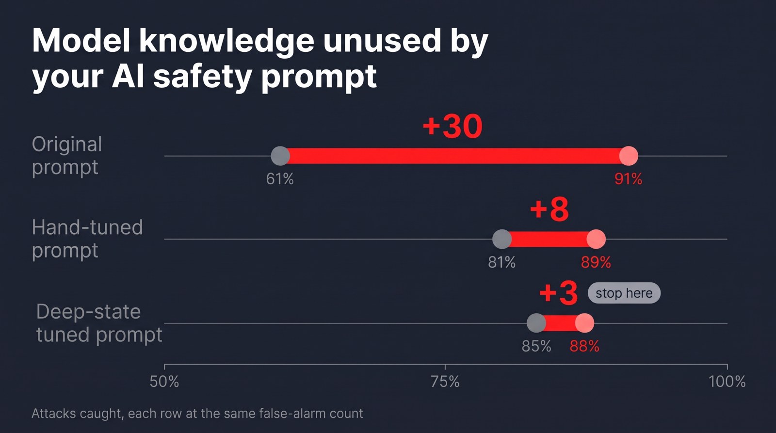
- Production prompt: judge 0.82, regression 0.97. Unused: 0.15.
- Hand-tuned prompt: judge 0.94, regression 0.98. Unused: 0.04.
- Best prompt: judge 0.97, regression 0.98. Unused: 0.015.
Look at the middle column first. The regression scored about the same under all three prompts. The information was in the model from the start, under the worst prompt nearly as much as under the best.
Now the first column. The judge’s own score went from 0.82 to 0.97. So the prompt did not make the model smarter. It decided how much of what the model already had reached the answer.
And the last column is the instruction. 0.15 unused: this prompt is worth optimising. 0.015 unused: about the size of wording noise, measured below. Stop.
Layer by layer the picture is the same. A regression fitted at each of the model’s 30 layers finds most of the information in place by layer 9, and the best any layer can do differs by only 0.015 between the three prompts. The judge’s answer differs by 0.096. The signal also sits in much the same place whatever the prompt says: a regression fitted under the production prompt and applied unchanged to the states produced under the other two still scores 0.90, 0.88 and 0.90 on held-out items. (Both measurements are on the tuning data, in full precision.)
For the record, the regression is class-balanced and L2-regularised, on the 2,816 numbers of the final state, fitted on the tuning set under the same prompt it is compared with. The three unused parts carry 95 % intervals from a paired bootstrap over test items: 0.154 [0.134, 0.175], 0.039 [0.027, 0.053] and 0.015 [0.007, 0.023]. Small under the best prompt, but not zero.
How many labelled examples it takes
Fewer than expected. The regression was refitted on random samples of the tuning set, ten times per size, and scored on the test set. Unused part under the production prompt and under the best one:
- all 1,579 examples: 0.15 and 0.015;
- 800: 0.144 and 0.011;
- 200: 0.116 and 0.005;
- 100: 0.082 and −0.002;
- 50: 0.039 and −0.012, with single draws all over the place.
Two things follow. A small sample makes the regression weaker, so on average the reading errs low: it understates what is unused. A single small draw can come out a little high, but never by much here. And the verdict that matters, large or small, was already clear at 100 to 200 examples. Shrinking the scoring set too, to 200 fitted and 200 scored, the production prompt read 0.11 give or take 0.03 and the best prompt 0.005 give or take 0.013.
What a small set cannot do is the fine work. The hand-tuned prompt’s 0.04 showed up only from 400 examples on; at 200 it read 0.008 give or take 0.025. And telling a real +0.015 from a +0.002 that is noise took the full test set.
Can wording really lose that much?
It can. On the tuning set, 25 wordings were scored both ways. The regression on the state came out at 0.945 with a standard deviation of 0.007. The judge’s own answer: 0.915 with a standard deviation of 0.021, three times as variable. (These two are AUC averaged within each data source, so they sit lower than the figures above.)
Then came answer words chosen backwards, so that a calm word meant “flag it”. A quick screen had predicted the judge would simply rank in reverse. Instead its score fell to 0.59, close to a coin flip. The regression on the very same states still scored 0.97.
That is the case accuracy alone cannot diagnose. A judge at 0.59 looks like a model that cannot do the task. It was a model that could, behind two badly chosen words.
Where the prompt does its work
One experiment went looking for the place. It swapped the model’s internal state at the answer position between a run with the production prompt and a run with the best one, layer by layer, and measured how much of the score difference came along. At layer 9 of 30: 5 %. At layer 15: 42 %. At layer 19: 83 %. The prompt’s effect enters the decision in the middle third of the network.
The route depends on the length of the page. On short pages the answer position reads the instructions directly, and that carries about 60 % of the effect. On long pages most layers cannot see back that far. Only 5 of Gemma’s 30 layers attend to the whole text; the rest look through a 1,024-token window. There direct reading carries 7 %, and the instructions arrive second-hand, through what they did to the page tokens on the way. (This was measured on 80 items.)
What closed the gap
Two rounds of prompt work.
The first took the judge from 0.82 to 0.94: frame the text as untrusted content handled for a user, and spell out the criteria.
The second took it from 0.94 to 0.97, and it was the unglamorous kind. Read the judge’s errors, the ones the regression got right, group them, and write decision rules from the groups. A site banner written for human visitors is not an attack. Text that tells an agent what to click, type or open is.
In words the prompt went 47 → 141 → 135. The second round made it shorter, not longer.
Taking the best prompt apart shows what each part is for. It has seven clauses, and each was deleted in turn on the tuning set. Two narrow triggers each protect one family of attacks. Without the clause about sending something to an address, recall on email-style attacks drops by 0.12. Without the clause about making an agent act before or instead of its own task, recall on web-agent attacks drops by 0.16. Three clauses do nothing measurable, and one of them is the banner rule quoted above. The clause that carries most is the least specific one, the opening sentence that sets the judge’s role: without it, benign pages flagged in one benchmark go from 4 to 47. And no single deletion moves the overall score beyond wording noise. The prompt works as a whole, and a rule that reads well is not evidence that it does anything.
From the production prompt to the best one, on the test set: attacks caught went from 61 % to 85 %, and real pages flagged by mistake from 68 to 13 of 864.
The greedy part
The best prompt had come from errors the regression got right. Was that choice the reason it worked? If so, the regression would be more than a gauge. It would say what to read next.
It looked plausible. Errors the regression gets right really are more fixable: later prompts fixed them 74–89 % of the time, against 31–39 % for the rest. So I tested it on the best prompt’s remaining mistakes. Eight LLM readers each read 80 errors and wrote new prompts. Two got errors the regression gets right, two got errors a plain text classifier gets right, four got random ones.
On the test set, prompts written from the regression’s picks were no better than prompts written from random errors. None of them beat the best prompt.
Knowing that an error is fixable turned out not to be the same as knowing the fix.
And once the unused part was small, nothing else found more either. An LLM proposed nine rewrites per round for four rounds: +0.015 on the tuning set, +0.002 on the test set. Few-shot examples picked by the regression came out ahead of random picks by less than wording noise.
There is also the opposite case, the one no wording will reach. On the tuning set the best prompt still missed 162 attacks. For 60 of them, all from one public benchmark, a probe was tried at every layer, and almost none were told apart from clean text at any depth. That is not a hidden ability. Either the model lacks it, or the labels mark a difference the text does not carry: the same banners appear on pages labelled attack and on pages labelled clean.
Two rules against false wins
That +0.015 that turned into +0.002 shows why both are needed.
Measure wording noise first. The best prompt was rewritten five ways with the same meaning. The six versions had a standard deviation of 0.016, with 0.041 between best and worst. That is how much the score moves when nothing has changed except the phrasing, so a change counts only if it beats twice the standard deviation.
Decide on data you did not tune on. The search gain shrank about tenfold on the test set. The best gain from error reading fell from +0.013 to +0.002. On the tuning set both had looked like progress.
What you can use from this
1. Set the check up once.
- A labelled set to tune on, and a second one collected afterwards and kept for scoring. A few hundred examples are enough to tell a large unused part from a small one. Keep a large set for the last step, choosing between prompts that differ by a hundredth.
- Final hidden state at the last token, from your serving software. llama.cpp: the embeddings endpoint.
- A class-balanced, L2-regularised logistic regression, refitted for each prompt you compare.
- Two numbers per prompt: the regression’s score and the model’s own. Their difference is the unused part.
2. Read the result.
- Large unused part (here 0.15): the model has it and the wording loses it. Prompt work will pay.
- Unused part near your wording noise (here 0.015 against 0.016): stop rewriting.
- Errors that no layer separates: wording is unlikely to reach them. They need something other than a rewrite, or the labels need a second look.
3. When the prompt is worth working on. Read the errors, group them, turn the groups into decision rules. That is what moved this judge from 0.94 to 0.97. Picking the errors with the regression, automated search and regression-picked few-shot examples added nothing measurable on top.
4. Guard against false wins.
- Rewrite your prompt five ways with the same meaning. The standard deviation of the scores is your noise. Count a change only beyond twice that.
- Score finalists on data collected after tuning. Tuning-set gains here shrank seven- to tenfold.
- If answers are single words, choose words whose plain meaning matches the decision. A reversed pair dropped this judge to 0.59 with the information fully intact.
5. Know what the check is not. It needs a self-hosted model and labelled examples. It says how much is unused, not how to use it. And a text classifier that never sees the model, built on character n-grams, scored close to the regression on the tuning set. Part of what the regression reads is surface wording, so treat its score as a mark to aim at, not as the model’s mind.
All of this is one model and one task.
Method, tables and confidence intervals: llm-judge-weights-probes-prompts